Cholesky (LDLT) Decomposition of a symmetric positive definite matrix using MPI

Introduction

This project was done as the final assignment for course 4810-1115 Parallel Numerical Computation. The course dealt with parallelizing numerical algorithms using OpenMP (shared memory parallelization) and MPI (distributed systems).

Problem statement

Given a symmetric positive definite matrix

\[A=\begin{bmatrix} a_{11} & a_{12} & a_{13} & \cdots & a_{1n}\\ a_{21} & a_{22} & a_{23} & \cdots & a_{2n}\\ \vdots & \vdots & \vdots & \ddots & \vdots\\ a_{n1} & a_{n2} & a_{n3} & \cdots & a_{nn} \end{bmatrix}\]

factorize it in two matrices

\[L = \begin{bmatrix} 1 & 0 & 0 & \cdots & 0\\ l_{21} & 1 & 0 & \cdots & 0\\ \vdots & \vdots & \vdots & \ddots & \vdots\\ l_{n1} & l_{n2} & l_{n3} & \cdots & 1 \end{bmatrix}\]

and

\[D = \begin{bmatrix} d_{11} & 0 & 0 & \cdots & 0\\ 0 & d_{22} & 0 & \cdots & 0\\ \vdots & \vdots & \vdots & \ddots & \vdots\\ 0 & 0 & 0 & \cdots & d_{nn} \end{bmatrix}\]

such that \(A = LDL^T\)

Algorithm

Values of the $L$ and $D$ matrices can be calculated using the following formulae

\[l_{ij} = \frac{a_{ij} - \sum_{k=1}^{j-1}d_{kk}l_{jk}l_{ik}}{d_{jj}}\] \[d_{ii} = a_{ii} - \sum_{k=1}^{i-1}d_{kk}l_{ik}^2\]

Sequential Code

The formulae given above can be very easily implemented into code. The code that I used in my report is as follows

void ldlt_sequential(const double* const A, double *L, double *d, const int n)
{
    // Fill upper part with zeroes
    for (int r=0; r < n - 1; ++r)
    {
        std::fill(L + r * n + (r + 1), L + (r + 1) * n, 0.0);
    }
    for (int j=0; j<n; ++j)
    {
        d[j] = A[j*n+j];
        for (int k=0; k<j; ++k)
            d[j] -= d[k] * L[j*n+k] * L[j*n+k];
        
        L[j*n+j] = 1;
        for (int i=j+1; i<n; ++i)
        {
            L[i*n+j] = A[i*n+j];
            for (int k=0; k<j; ++k)
                L[i*n+j] -= d[k] * L[j*n+k] * L[i*n+k];
            L[i*n+j] /= d[j];
        }
    }
}

Parallelization using MPI

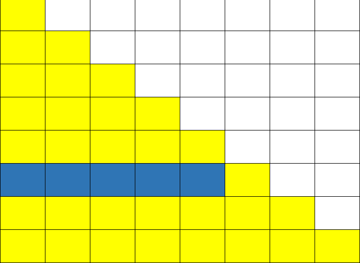Figure 1: Data needed from $L$ to calculate an element of $D$

Figure 2: Full rows $i$ and $j$ of $L$ are needed to calculate $L[i, j]$

Data Dependencies

We can see that in the calculations, every column of $L$ and $D$ needs the values of their previous columns already calculated, however calculation of rows can be done a bit independently.

$D$ Matrix

For $D$, we can see from the equations that to get any element of $D$ we need all its previous elements and the complete row of the matrix $L$. We can see the dependency in figure 1, where dark blue columns are the ones which are needed.

$L$ Matrix

If we are calculating say column $i$, than we need all the previous values of $D$ and the complete row $i$ of $L$. In the figure 2, we can see that for calculation of $L[r, 4]$ we need $L[4, :]$ and $L[r, :]$.

How the parallelization is done

Since every column needs the values of its previous columns so there is not an easy way to parallelize that, so I have gone through all columns in sequential manner but in every column I have divided the work for rows to different processes.

Calculating $d_{ij}$

Every rank is resposnsible for calculating values of rows that are multiple of rank. In this way the value of $D$ can also be divided among processes because it already has the previous computations from that row so it does not need any data to be communicated to it for calculation of $d_{ii}$. After calculation the values of $d_{ii}$ are sent to all other processes since it will be needed for calculation of $L_{ij}$.

Calculating $L_{ij}$

As soon as we start to calculate the values of a column, say column $j$, we broadcast the $j^{th}$ row to all the processes since it is needed as shown in figure 2. All the processes do their work independently and at the last they update the values when they receive the value of $d_{ii}$. They do not send the calculated values anywhere at this point of time, so there is no communication overhead.

Parallelized code using MPI

void ldlt_mpi(const double *const A, double *L, double *d, const int n)
{
    int rank, n_pr;
    MPI_Request req_for_row, req_for_dj;
    MPI_Comm_rank(MPI_COMM_WORLD, &rank);
    MPI_Comm_size(MPI_COMM_WORLD, &n_pr);

    // Fill with zeroes
    std::fill(L, L + n * n, 0.0);

    // Have to go column wise, can not be parallelized
    for (int j = 0; j < n; ++j)
    {
        L[j * n + j] = 1;

        // This row is needed by everyone so start sending it
        MPI_Ibcast(L + j * n, j, MPI_DOUBLE, j % n_pr, MPI_COMM_WORLD, &req_for_row);
        if (j % n_pr == rank)
        {
            d[j] = A[j * n + j];
            for (int k = 0; k < j; ++k) 
                d[j] -= d[k] * L[j * n + k] * L[j * n + k];
        }
        // Value for d[j] will be needed by every row so start sending it
        MPI_Ibcast(d + j, 1, MPI_DOUBLE, j % n_pr, MPI_COMM_WORLD, &req_for_dj);
        // Now the row is needed to compute values
        MPI_Wait(&req_for_row, MPI_STATUS_IGNORE);

        // Distribute the work for rows
        for (int i = j + 1; i < n; ++i)
        {
            if (i % n_pr == rank)
            {
                L[i * n + j] = A[i * n + j];
                for (int k = 0; k < j; ++k)
                    L[i * n + j] -= d[k] * L[j * n + k] * L[i * n + k];
            }
        } // work for each row ends

        MPI_Wait(&req_for_dj, MPI_STATUS_IGNORE);
        for (int i = j + 1; i < n; ++i)
            L[i * n + j] /= d[j];
    } // work for each column ends
} // function ldlt_mpi ends

Verification of Results of Parallel Code

For verification that the result obtained using parallel algorithm are correct, I have simply used the product $LDL^T$ and checked it against $A$, which was found correct for all the combination of MPI processes and matrix sizes. Matrix multiplication was done sequentially.

Performance

The code was run for various combination of matrix sizes and number of MPI processes and considerable speedup was seen both in terms of strong and weak scaling. Complete results are shown in table 1.

Table 1: Running time (in ms) for different values of MPI process and matrix sizes

Mat size	Sequential	Parallelized using MPI (number of processes)
		2	4	8	16	32	40	64	80	128	256	512
100	0.7	1.1	1.27	2	2.96	4.7	6.7	16.3	20.4	23.75	27.4	28.2
200	5.6	4.63	3.58	4.1	4.95	6.65	7.9	13.67	13	26.83	54.2	53.65
500	86.8	50	30	24	22.2	23.85	25	49.1	75.3	95.34	101.7	163
750	293.4	159	89	60	47.7	45.24	48	48.27	46	70.3	214.7	159
1000	696.2	367	199	123	85.9	75.3	75	76.3	72	81.4	137	332
1500	2490	1215	638	363	227.8	180	178	169.14	148	160	159	437
2000	6234	2901	1477	806	477	361	348	300	257	273.5	261	472
2500	12124	6057	2876	1537	905	660	622	494	412	416	397	672
3000	20767	10482	5062	2715	1569	1056	981	763	612	618	579	940
3500	32733	16588	8217	4357	2425	1536	1397	1111	860	869	786	1241
4000	48573	24454	12376	6527	3614	2239	1956	1551	1193	1197	1053	1604
5000	93340	47194	23773	12335	6658	4015	3512	2840	2248	2251	1769	2504

Weak Scaling

From table 1 we see that upto a certain level (approximately till $64$ processes) that increasing the number of processes allows us to solve bigger and bigger problems. For example in the sequential algorithm we can solve the problem with matrix size of $750 \times 750$ in around $300ms$, while with $64$ processes we can solve the problem for matrix size of $2000 \times 2000$ in the same time. In the figure 3 it is clearly seen that execution time decreases with increasing parallelism.

Strong Scaling

It is clearly seen that offering more processors helps us solving the problems faster (if they are big enough to be benefitted from parallelization). For the matrix size of $5000 \times 5000$ the sequential algorithm takes $93340ms$, which is around $1.6$ minute, which using $80$ processes in parallel, the same problem is solved in less than $2.3s$. This can be seen in table 2 and figure 4.

Matrix Size	Speedup by parallelization for different number of MPI processes
	2	4	8	32	64	80	128	256	512
100	0.64	0.55	0.35	0.15	0.04	0.03	0.03	0.03	0.02
200	1.21	1.56	1.37	0.84	0.41	0.43	0.21	0.10	0.10
500	1.74	2.89	3.62	3.64	1.77	1.15	0.91	0.85	0.53
750	1.85	3.30	4.89	6.49	6.08	6.38	4.17	1.37	1.85
1000	1.90	3.50	5.66	9.25	9.12	9.67	8.55	5.08	2.10
1500	2.05	3.90	6.86	13.83	14.72	16.82	15.56	15.66	5.70
2000	2.15	4.22	7.73	17.27	20.78	24.26	22.79	23.89	13.21
2500	2.00	4.22	7.89	18.37	24.54	29.43	29.14	30.54	18.04
3000	1.98	4.10	7.65	19.67	27.22	33.93	33.60	35.87	22.09
3500	1.97	3.98	7.51	21.31	29.46	38.06	37.67	41.65	26.38
4000	1.99	3.92	7.44	21.69	31.32	40.72	40.58	46.13	30.28
5000	1.98	3.93	7.57	23.25	32.87	41.52	41.47	52.76	37.28

Conclusion

The problem was successfully parallelized using MPI and almost linear speedup was seen for sufficiently large problem where computations were more than communication overheads.

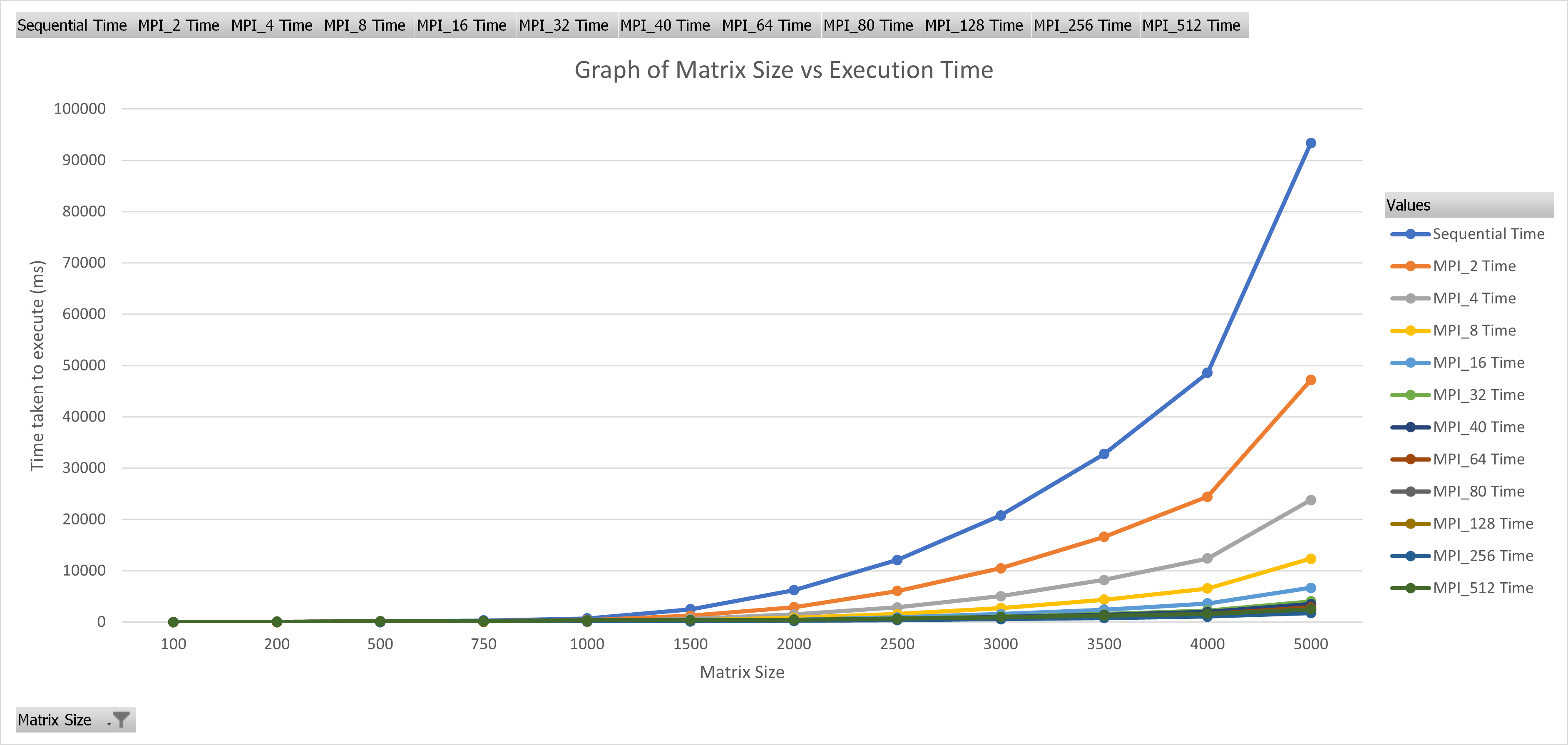Figure 3: Matrix size vs execution time for various number of MPI processes

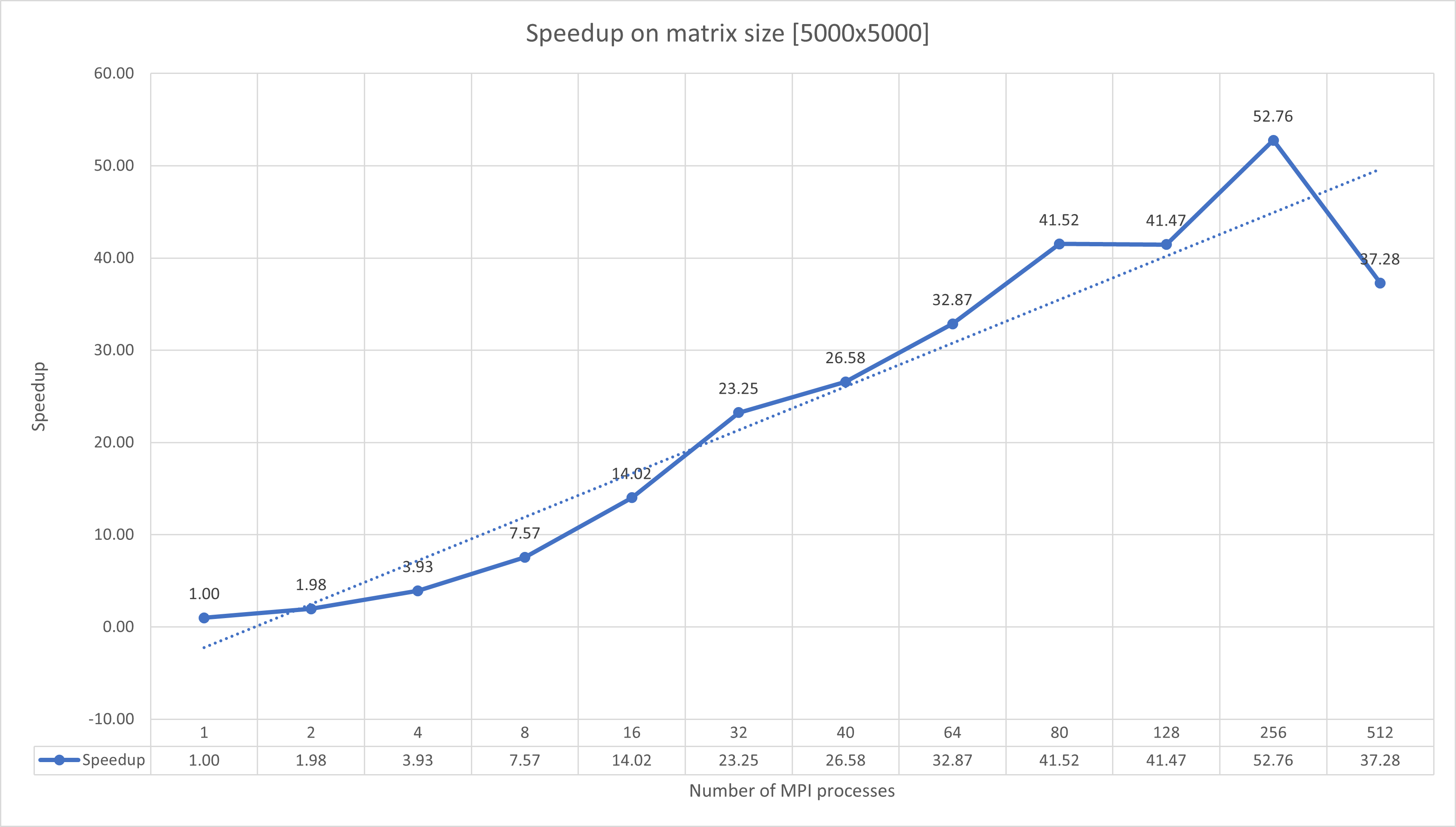Figure 4: Speedup of $5000 \times 5000$ matrix with different number of MPI processes

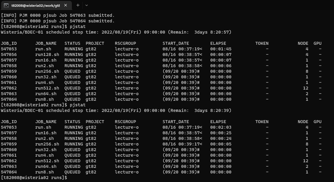Figure 5: Snapshot of submission using pjstat